Simulation of a motor control system at different levels of detail

Numerical simulations are a part of any design today, the same can be said for control systems and electronics design
The level of depth and detail in a simulation will be a major factor in deciding which effects and phenomenon are we able to capture in the simulations and which we missed
This decides how accurately the simulations model the physical hardware

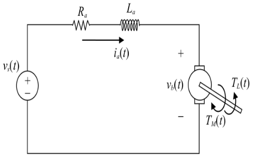
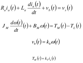
Let’s simulate the motor control system with following dynamics

First order transfer function

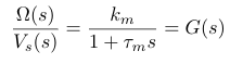
Speed , in the Laplace domain , after neglecting the armature inductance

Transfer function from volt to speed

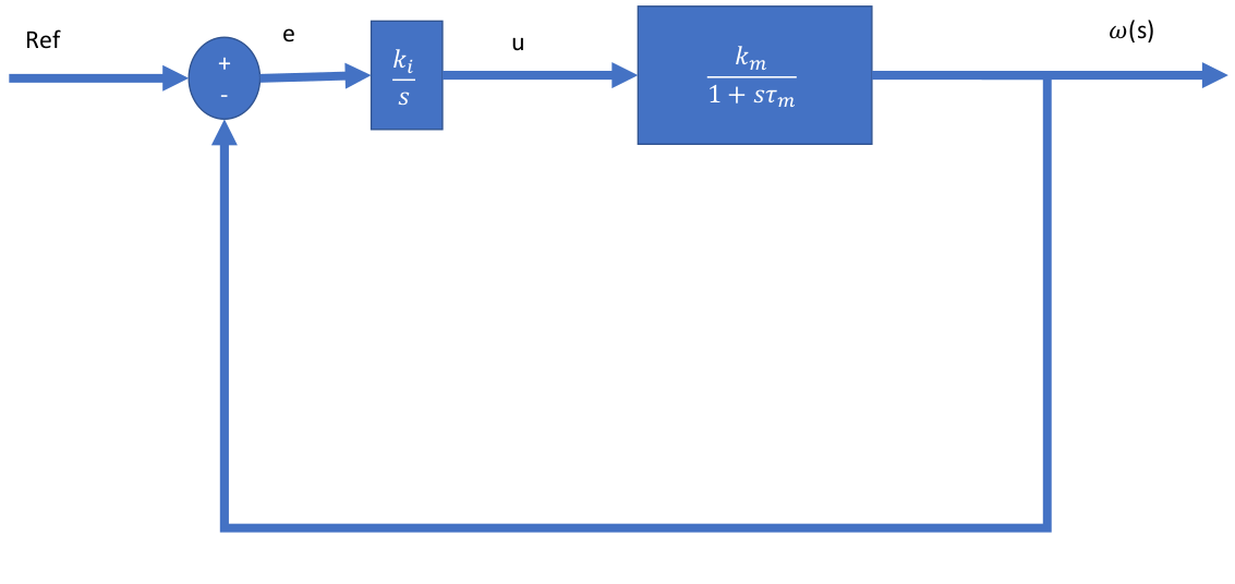
Feedback control of motor (modelled as a first order transfer system)

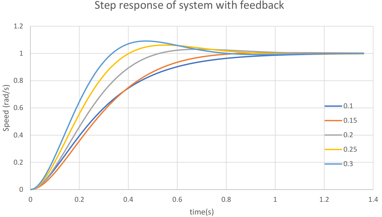
Step response of a feedback system (with different values of compensation gain Ki)

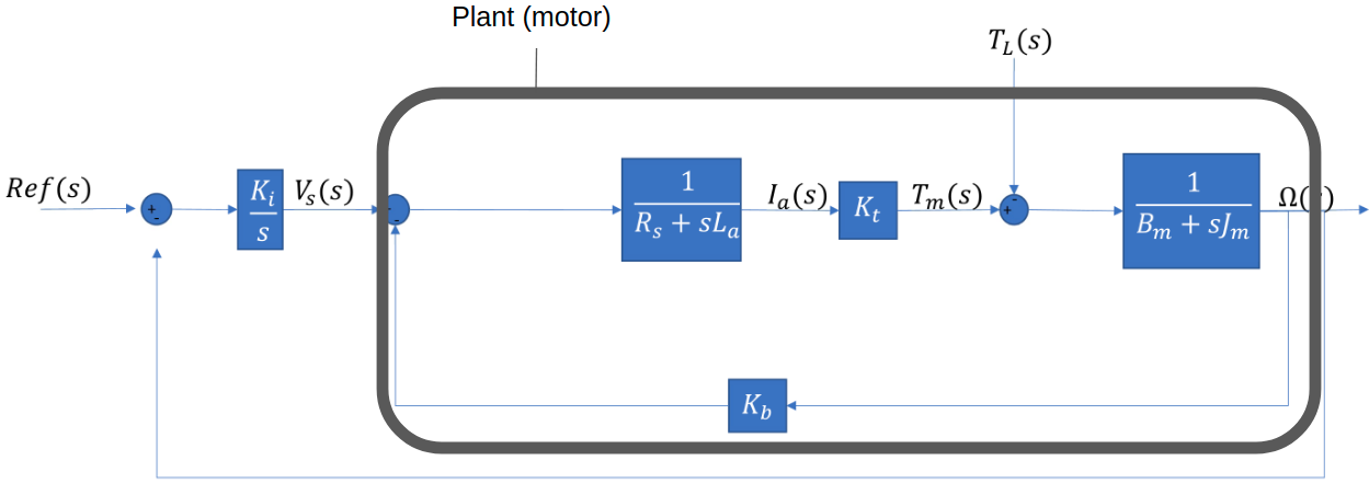
Second order Model with feedback

Unit step response

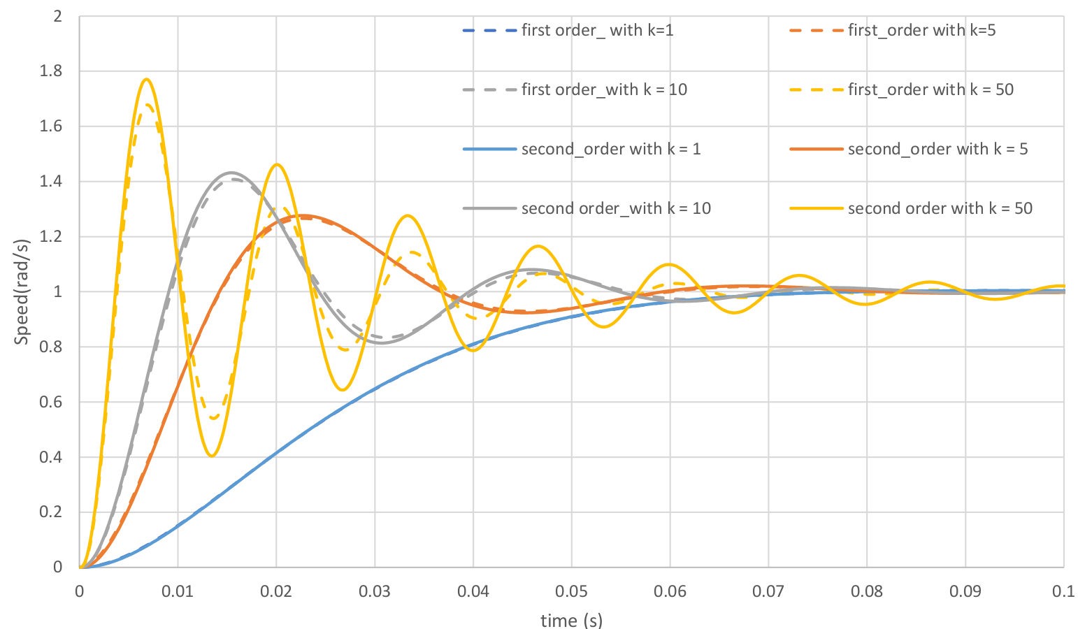
There is a slight difference in the response at higher values of compensation gain

Stability analysis

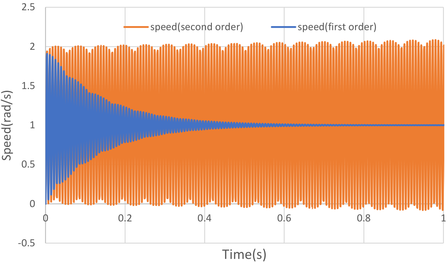
At a compensation gain Ki of 1600
The second order model gives sustained oscillations whereas the first order does not

The first order model is always stable and cannot be used for stability analysis

Micro-controller based control

In reality the control would be implemented in
software using a micro-controller.
The physical system would something like :

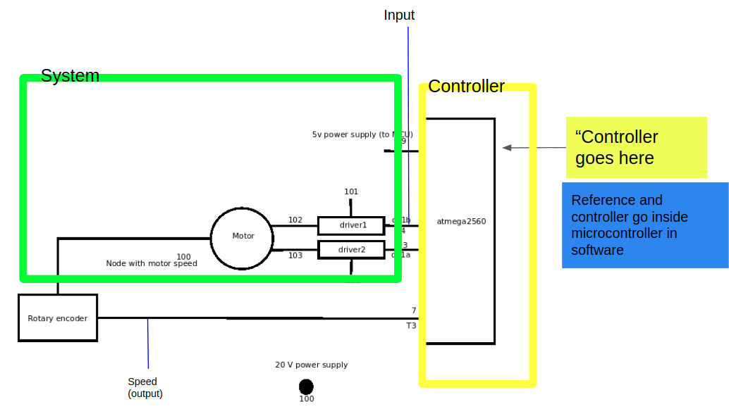
The C-code implements the control system and the exact software (compiled binaries) are used for simulation

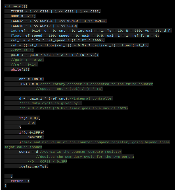
A micro-controller will update the output and sense the input after a sampling period Ts. This sampling period also will have an effect on the output of the system.
The effect of the PWM signal (see the right figure) and sampling time can be observed using tessim simulations.

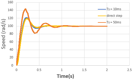
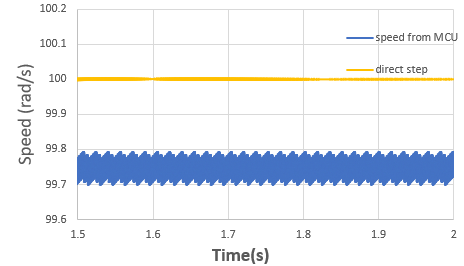
Effect of motor driver

The motor driver will have some delays in giving the output and some finite ramp times .
These delays would introduce a "dead-band" in the motor speed at lower values of duty cycle.
‍

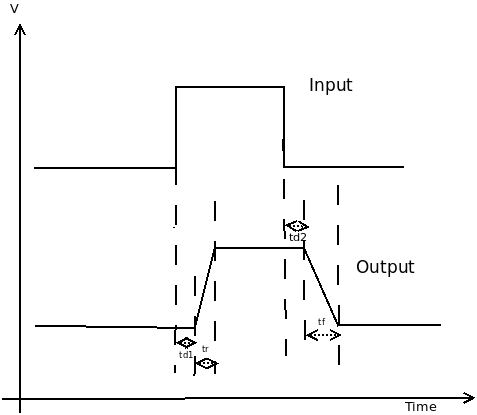
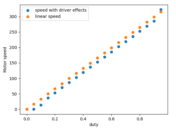
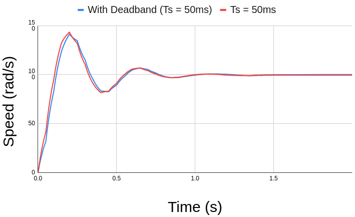
Effect driver effects (dead-band)

       1. There will be a slight difference in the response with and without dead-band
‍
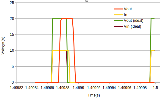
       2. Input and output PWM signals for motor driver in ideal and non-ideal case
‍
       3. After including the delays from the driver , the input duty cycle (output from MCU) is slightly larger than the ideal case. This is because for the same duty cycle we get lower speed, so for the same speed, a higher duty cycle would be required. This can be seen in the ideal and the actual plots of PWM signal below.

Overall conclusion

First order approximation :
get average steady state speed, accurate at low value of compensator
Second order approximation:
Stability analysis : The first order system is always stable, we need a second order model for stability analysis
does not show the effect of PWM signal and sampling time
Microcontroller with an ideal driver :
effect of PWM signals , sampling time and digitisation
Testing the exact software for simulation purpose
Driver delays :
Effects of driver parasitics like delays and ramp up/down times.

Simulation at different levels